Session 5
August 24, 2023
Agenda
- dplyr continued
- Create new variables with
mutate() - Group data using
group_by() - Create (grouped) summaries with
summarise()
Resources
We will continue to talk about things covered in Chapter 5, this time sections 5.5 - 5.7.
The kableExtra package is great for styling tables
created by for example summarise(). Information about this
package can be found here.
Homework Exercises
The session 5 homework is below. All code solutions should be completed using one (sometimes rather long) pipeline.
Recreate the code to make the plot below. Make sure your code includes the fix we talked about during the Thursday session to correct the Weight observations made by
raID-07.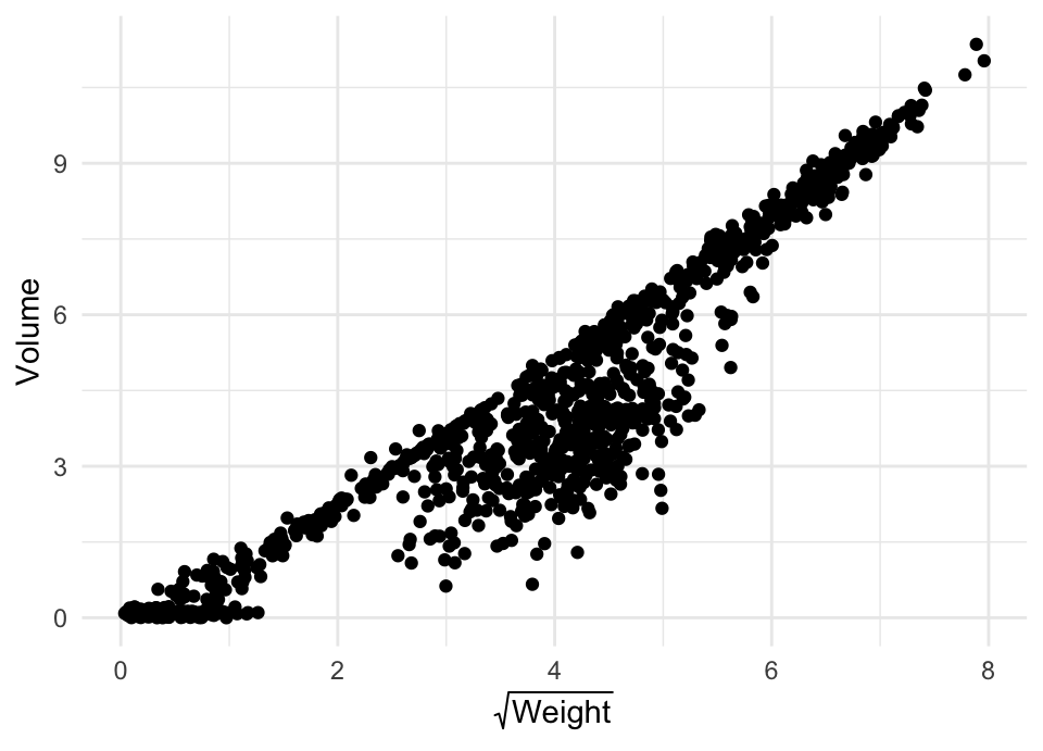
Use
group_by()andmutate()to calculate the median Volume per Observer, and call the new columnmedian_Volume.Find the largest Volume measurement per phase, using
group_by(),summarise()andmax().How many observations per phase has a Weight less than 10 grams?
Mean-center (subtract the mean from all the individual observations) the
Weightvariable (corrected). What is the mean of this new variable?Mean-center the Volume variable for each phase separately.
Recreate the plot below, but instead of asking
geom_bar()andgeom_errorbar()to calculate the mean and the standard error, calculate these values yourself usinggroup_by()andsummarise(). Once these summary statistics are calculated, pipe toggplot()and add the code necessary to produce the plot. Use google to figure out how to calculate standard errors and how to use pre-calculated values withgeom_errorbar().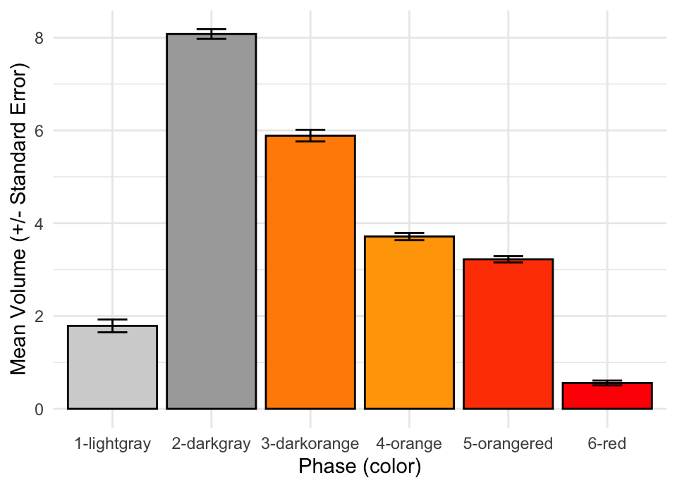
Using the plot above as a starting point, create two new plots; one with errorbars representing the median absolute deviation and one with errorbars representing 95% confidence intervals.
During session 4, we talked about how to use the
DTpackage to create interactive tables. These are perhaps most suited for large tables where showing all information would be problematic without the ability to produced paged, clickable tables. Many times when working in R we produce smaller tables, which is often the case when workinggroup_by()andsummarise()for example. Out of the box, these tables don’t look very good when knitting a html document. Check the resources and see if you can reproduce the code necessary to make the table below.Table 1: Cloudbuddy Volume
Phase (color)
mean
stdev
n
1-lightgray
1.79
1.95
199
2-darkgray
8.08
1.49
202
3-darkorange
5.89
1.77
199
4-orange
3.71
1.09
196
5-orangered
3.22
0.94
199
6-red
0.56
0.72
191
Calculate the difference in mean Volume between observations younger than the median age and observations older than the median age.
Focusing on the first two observers, calculate the proportion of observations done per phase by each observer out of the total number of observations made by each observer. When you are done, the output should look like the table below.
Observer
Phase (color)
Proportion
raID-01
1-lightgray
0.1638418
raID-01
2-darkgray
0.1807910
raID-01
3-darkorange
0.1581921
raID-01
4-orange
0.1581921
raID-01
5-orangered
0.2033898
raID-01
6-red
0.1355932
raID-02
1-lightgray
0.1618497
raID-02
2-darkgray
0.1791908
raID-02
3-darkorange
0.1618497
raID-02
4-orange
0.1734104
raID-02
5-orangered
0.1676301
raID-02
6-red
0.1560694